Big o notation socks

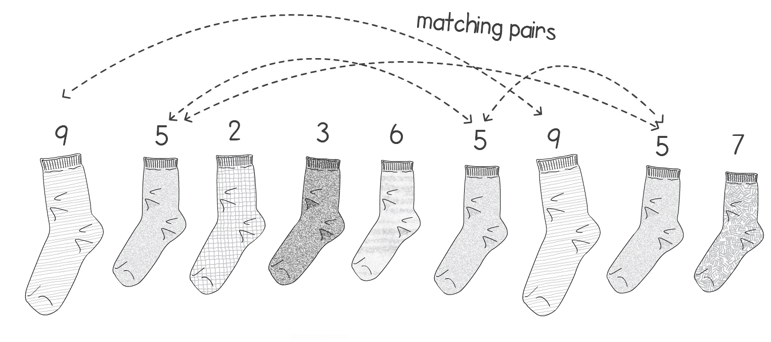
A few weeks ago I tweeted the following:
“Looking for matching pairs of socks in the morning is always an O(n²) task for me. Anyone got a better algorithm?”

I received a few responses which gave me the idea to use sock matching to explain big O notation.

Right. Let’s start from defining the problem.

Let’s assume we have n single socks and each matching pair is labeled with a number i. We define a pair of socks a and b as being a matching pair if

Here’s a picture of an example of what I mean with the value if i on top of the sock:

A couple of things to mention from the example picture above:

1. Some socks do not have a matching pair. In the above that is 2, 3, 6 and 7. On some days I swear there is a one legged thief doing this…
2. Some socks can match with more than one sock, such as socks with label 5. This happens when you buy a bundle of socks of the same type and colour.

The aim here is to find any one matching pair. Think about when you wake up in the morning, open your sock drawer and need to find a pair that matches before going to work.

If we had to write some code to represent this problem we could put the sock labels in a collection and feed it to a function that returns the label of any match found or a -1 if no match is found. A return of -1 means you’ll be going to work with flip flops.

There are various approaches we can take in order to solve our problem. But how do we know which one is the best? And what does “best” even mean? If you’re like me and your mornings are always a bit of a logistical challenge, the “best” means the fastest way I can get out of the house. 

The problem is that speed is a slippery concept when it comes to algorithms. An algorithm might be fast in one type of input but perform poorly with another. So using speed alone is not a good indication. To go around this problem, in computer science, we don’t measure speed but scale. We ask the question: How bad will the program degrade as I increase the size of my input? The lower the degradation the better the algorithm will scale to larger inputs. To describe this, we use what is known as the Big O notation. The following sections try to give you an intuition of how we measure this by going through various examples.
​

The Quadratic algorithm

Our first attempt to solve this sock matching problem would be the way most of us do it when we’re in a hurry (although it’s also the slowest!):

1. Pick the first one from the pile and keep it in your left hand.
   
2. Go through every other sock using your right hand and see if it matches with the one we’re holding in your left.
   
3. If no match is found, put the left hand sock away and start again from 1 until we go through every sock.
   

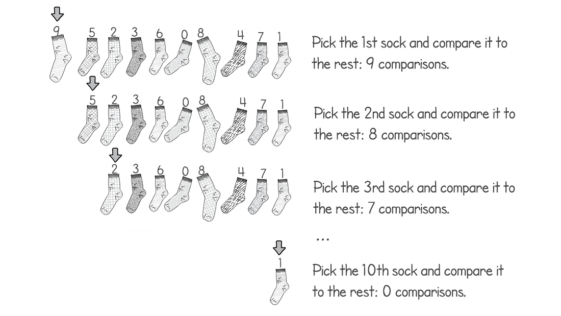
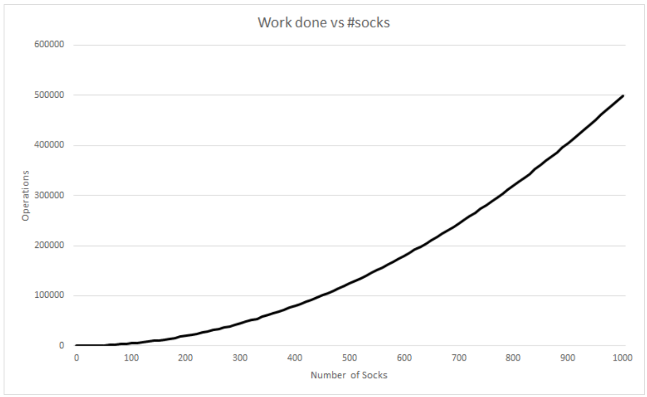
In python this can be written as:

Say we have 10 socks in our pile. How many sock comparisons would we have to do with this setup? 

Of course that depends on the contents and way the pile is organized. If we’re lucky we’ll find two matching socks on the top of the pile, in which case we would only need to do one comparison (comparing the first two socks). This is called the best case scenario of an algorithm. Our best case does not change whether we had 10 or 1 million socks. If the first two socks match, we’ll always do one comparison. Although the probability of the best case occurring with 1 million socks is lower than 10 socks.

The problem is that the best case doesn’t really tell us much about how good our technique is. We might be lucky a couple of times but it’s unlikely we’ll have the best case occurring every day in the long run, especially if we keep many socks. So we need another way to compare how good our solution is.

Whenever we quote the Big O notation of an algorithm, typically we are referring to the worst case of the algorithm (although the average case is also used sometimes). The worst case is a much more useful measure to use to compare different approaches. If we know that an algorithm A is, in the worst case, better than algorithm B it will give us a better idea that A will perform better than B.

This is the first rule when you come to compare algorithms using Big O notation. Use the worst case scenario. Sometimes you also want to compare the average case, but for the purpose of this article we’re sticking with the worst as it’s easier to understand and it’s usually enough.

Right, can you think of the worst case scenario of our solution listed above? The worst case is when there isn’t a single matching pair in the pile. This is when you’re going to get to work late wearing mismatched socks. Now, for this worst case, try to work out the number of sock comparisons we need to perform if we had 10 socks at the start.
​

So in total we would have done 9 + 8 + 7 + 6 + 5 + 4 + 3 + 2 + 1 + 0 comparison operations. If you sum this up it would give you 45.

What if we had 100 socks instead of 10? This would result in 99 + 98 + 97… + 0 sock comparisons. There is an easy formula that would give us the result of this sum, without having to do the entire calculation:

If we had to generalize for when we have an arbitrary number of socks n, we have:

If you’re interested in how I got to the above expression, have a read through the wiki page: en.wikipedia.org/wiki/1_%2B_2_%2B_3_%2B_4_%2B_%E2%8B%AF#Partial_sums
Fun fact: The above equation would also give you the total number of handshakes that would happen in a meeting with n people.
​
What does this tell us about how good our algorithm is? Notice that when we increased the input (number of socks) by a factor of 10, from 10 to 100, our effort did not increase proportionally. For 10 socks we have to do 45 operations, however for 100 socks that number is 4950, not 450. How about we plot a chart with the input size vs the number of sock comparison operations we have to do?

The above chart shows how much extra work we need to do as we increase our input. If it took us one second to compare a pair of socks, it would take us 1hr 20 mins in the worst case for 100 socks. If we increase the number by a factor of 10 again (1000 socks) it would take us almost 6 days to find a matching pair.

So what is the Big O notation for our algorithm? We have already seen the expression that would give us the worst case scenario for this. We can expand that formula to give us:

There are only two rules to convert any expression into Big O notation. First you drop any constants and then you only consider the part with the highest order. In our example the highest order of our expression is the squared part. Thus the above would result in: 

In geek speak we say that our sock matching algorithm has a quadratic worst case time runtime complexity or simply a Big O of n squared. The reason why we simplify the expressions in this way is that as n gets bigger and bigger, the parts of the expression with the lower orders count less and less. In practise, our algorithm is a little faster than n2 however this advantage gets less noticeable for large values of n.
​

The Linear algorithm

How can we improve our sock matching? A friend of mine suggested keeping socks in some sort of order to make matching easier. This has never worked for me as the washing machine does a very good job of randomly shuffling them. For a moment let’s assume you do find a way to keep them sorted or maybe you order them as soon as they come out from the wash, how will our sock matching algorithm change?​

We can make use of the fact that the socks are sorted and we only need to match each sock to the one next to it. The algorithm would go something like this:

1. Pick the first sock in your left hand
   
2. Pick the next sock in your right
   
3. If the socks in your left and right hand match then you have found a match
   
4. Otherwise, If there are more socks 
   
   1. get rid of the sock on the left hand
      
   2. move the right hand sock to the left
      
   3. Repeat from step 2
      

In python this can be written as:

How does this affect our runtime performance? Again let’s think about our worst case performance, i.e. when we do most work. Again in this case this is when we cannot find a match and go through all of the socks. How many steps do we take? Let’s try to be more precise here. For almost each sock, we pick it up with the right hand, do a comparison and then pass it on to the left hand, i.e. 3 steps per sock. This means that if we had n socks the number of steps we take is:

Now remember that to convert the above to Big O notation, we need to drop the constants and take the highest order. In this case we end up with:

Notice that to derive the complexity of an algorithm we don’t have to be precise and count every single operation that the algorithm makes. If we only counted the sock comparisons instead of the picking up the socks in your hand, we would have arrived at the same expression. The important thing here is that we are consistent, we choose what to count and stick with it.

This is what is called an algorithm with a linear runtime complexity and is usually what our mind defaults to when it thinks of proportions. Put simply, if you double the input size (number of socks) you also double the total number of operations. If it takes us 1 second to compare a pair of socks, it would take us 1000 seconds for 1000 socks, as opposed to the 6 days for the quadratic solution. Quite an improvement!
​

Constant algorithm

Can we improve even further? Another friend suggested that I throw away all my socks and buy many socks of the same type, colour and size. Genius and boring I thought… ​
​

Our algorithm will now be very simple. Basically we just need to choose any two socks:

1. Pick the first sock in the left hand
   
2. Pick the second sock in the right hand
   

Any in python this would be:

How does our performance change as we increase our input? First of all notice that in this case the worst case of the algorithm is the same as the best. Also it doesn’t matter if we have a couple of socks or a million. We will always perform the same couple of operations and the algorithm will take the exact same time. This is what we call a constant complexity, written as:

A constant runtime complexity is the most scalable type and is usually the most desired type of algorithm. Notice that again it doesn’t matter how many operations we do in our algorithm as long as it doesn’t change when we change the input size. 

It’s worth mentioning that computational complexity doesn’t tell us how fast an algorithm works for a particular input. It might well be that a constant algorithm might work slower than a quadratic one for a certain small input. If we only had two matching socks, all of our matching methods will perform quite well. Big O notation only compares how well different approaches scale with the input size.

In our article we only explored three types of complexities, but there are many other types. Have a look at this wiki article to see all the different types of complexities:
en.wikipedia.org/wiki/Time_complexity